Stages of development of the robot-balancer

Stages of development of the robot-balancer

2014-04-26

Finally, I completed the construction of the robot balancer. For him, a mathematical model and a linear-quadratic regulator were calculated.
That's what happened, it can even be controlled from the phone:



First I tried to build a robot on a PID controller without any mathematics, but after several days of unsuccessful attempts to pick up the PID controller's coefficients, I gave up this venture.

Let's start by calculating a mathematical model.

Mathematical model

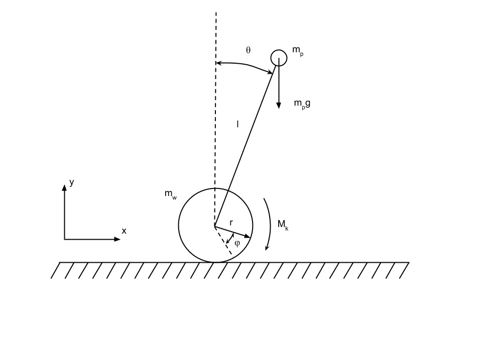
Consider the system inverted pendulum on the wheel, pictured above. We will Consider that the system moves without friction. The pendulum represents the mass m p , Attached to a weightless rod of length l to the wheel. The wheel is considered a ring Radius r and mass m w . The moment of the motor M k acts on the wheel M p : mass of the pendulum M w : mass of wheels L: length of the pendulum R: wheel radius Θ: angle between pendulum and vertical straight line Φ: angle of rotation of the wheel relative to its initial position M k : Motor torque

To investigate the system, we use the Euler-Lagrange equations.
$ \ Frac {d} {dt} (\ frac {\ partial L} {\ partial \ dot {q}} (q, \ dot {q})) - \ frac {\ partial L} {\ partial {q} } (Q, \ dot {q}) = \ tau $ (1.1)

We express the position of the center of the wheel through the rotation angle: $ X = r \ phi $. (1.2) We note that the coordinates of the center of mass of the pendulum are found from the following relations: $ X_g = x + l sin (\ theta) $ (1.3) $ Y_g = l cos (\ theta) $ (1.4) First we calculate the representation for the kinetic energy of the system. Kinetic The energy of the pendulum is
$ T_p = \ frac {1} {2} [m_p \ dot {y} _g ^ 2 (t) + m_p \ dot {x} _g ^ 2 (t)] $. (1.5)
The kinetic energy of the wheel is
$ T_w = \ frac {1} {2} [m_w \ dot {x} ^ 2 (t) + m_w r ^ 2 \ dot {\ phi} ^ 2 (t)] $ (1.6)
Substituting (1.2), (1.3), (1.4) into (1.5) and (1.6), we obtain the total kinetic energy
$ T = \ frac {1} {2} m_p l ^ 2 \ dot \ theta sin (\ theta) ^ 2 + \ frac {1} {2} m_p r ^ 2 \ dot {\ phi} ^ 2 + \ frac {1} {2} m_p l ^ 2 \ dot {\ theta} ^ 2 cos (\ theta) ^ 2 + m_w r ^ 2 \ dot {\ phi} ^ 2 + \ frac {1} {2} m_p l ^ 2 \ dot {\ theta} ^ 2 $ (1.7)
The total potential energy is
$ \ Pi = m_p gl cos (\ theta) $
The Lagrange function is given by the formula $ L = T- \ Pi $
Eventually
$ L = \ frac {1} {2} m_p l ^ 2 \ dot \ theta sin (\ theta) ^ 2 + \ frac {1} {2} m_p r ^ 2 \ dot {\ phi} ^ 2 + \ frac {1} {2} m_p l ^ 2 \ dot {\ theta} ^ 2 cos (\ theta) ^ 2 + m_w r ^ 2 \ dot {\ phi} ^ 2 + \ frac {1} {2} m_p l ^ 2 \ dot {\ theta} ^ 2-m_p gl cos (\ theta) $

We derive the equations of motion by means of Lagrange equations of the second kind (1.1). As generalized coordinates, let us take the angles of rotation of the wheel and the pendulum. Then The vector of generalized coordinates is represented in the form
$ Q = \ begin {pmatrix} \ phi \\ \ theta \ end {pmatrix} $
The generalized forces vector is as follows:
$ \ Tau = \ begin {pmatrix} M_k \\ 0 \ end {pmatrix} $
Substituting the derivatives into Lagrange's equations (1.1), we derive equations Movement :
$ R cos (\ theta) l m_p \ ddot \ theta + r ^ 2 (m_p + 2m_w) \ ddot \ phi-rsin (\ theta) \ theta ^ 2lm_p = M_k $ (1.5)
$ \ Ddot \ phi cos (\ theta) l m_p r-m_p gl sin (\ theta) + 2m_pl ^ 2 \ ddot \ theta = 0 $ (1.6)

The system can be given a standard look:
$ M (q) \ ddot q + C (q, \ dot q) \ dot q + G (q) = \ tau $, where
$ Q = \ begin {pmatrix} \ phi \\ \ theta \ end {pmatrix} $,
$ M (q) = \ begin {bmatrix} r ^ 2 (m_p + 2m_w) & r cos (\ theta) l m_p \\ r cos (\ theta) l m_p & 2 m_p l ^ 2 \ end {bmatrix} $ ,
$ C (q, \ dot q) = \ begin {bmatrix} 0 & -r \ dot \ theta sin (\ theta) l m_p \\ 0 & 0 \ end {bmatrix} $,
$ G (q) = \ begin {pmatrix} 0 \\ -m_pg l sin (\ theta) \ end {pmatrix} $ and
$ \ Tau = \ begin {pmatrix} M_k \\ 0 \ end {pmatrix} $

To control the resulting system, we construct a linear-quadratic regulator. To this end, we linearize the resulting equations of motion (1.5) and (1.6) in Neighborhood of the zero position of the pendulum: $ \ Frac {d} {dt} \ begin {bmatrix} \ phi \\ \ dot \ phi \\ \ theta \\ \ dot \ theta \ end {bmatrix} = AX + BM_k = \ begin {bmatrix} 0 & 1 & 0 & 0 \\ 0 & 0 & \ frac {-m_p g} {r (m_p + 4m_w)} & 0 \\ 0 & 0 & 0 & 1 \\ 0 & 0 & \ frac {g (m_p + 2m_w) )} {L (m_p + 4m_w)} & 0 \ end {bmatrix} \ begin {bmatrix} \ phi \\ \ dot \ phi \\ \ the \\ \ dot \ theta \ end {bmatrix} + \ begin {bmatrix } 0 \\ \ frac {2} {r ^ 2 (m_p + 4m_w)} \\ 0 \\ \ frac {1} {lr (m_p + 4m_w)} \ end {bmatrix} M_k $

The problem of optimal control is analyzed in detail in the book of Professor VN. Afanasyeva "Optimal control systems. Analytical construction ". In this article I will not dwell on it.

Control

The control I calculated with MatLab, there is an lqr function that calculates the coefficients.

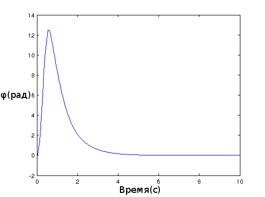
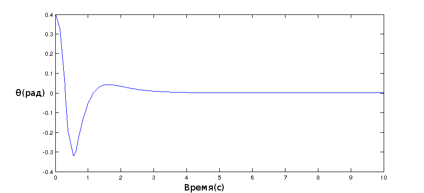
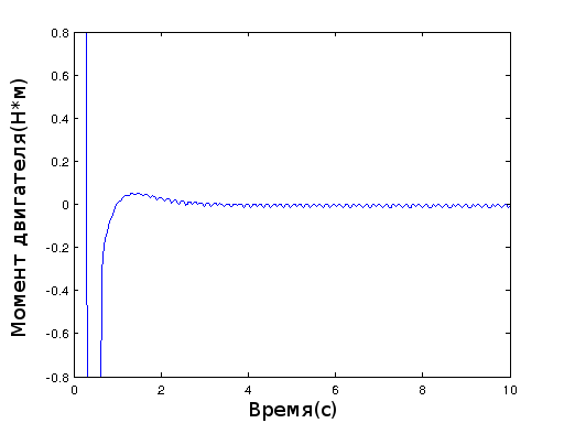
Modeling

Modeling produced in simulink and here's what happened:

Embodiment in iron

To calculate the angle, the data from the accelerometer and the gyro enter the complementary filter (RC filter).


float lastCompTime=0; float filterAngle=1.50; float dt=0.005;//0.002 //0.005 float comp_filter(float newAngle, float newRate) { dt=(millis()-lastCompTime)/1000.0; float filterTerm0; float filterTerm1; float filterTerm2; float timeConstant; timeConstant=0.5; // default 1.0 filterTerm0 = (newAngle - filterAngle) * timeConstant * timeConstant; filterTerm2 += filterTerm0 * dt; filterTerm1 = filterTerm2 + ((newAngle - filterAngle) * 2 * timeConstant) + newRate; filterAngle = (filterTerm1 * dt) + filterAngle; lastCompTime=millis(); return filterAngle; }
On the motors there are quadrature encoders, I was lazy to use interrupts and I copied the standard code from the examples arduino
void doEncoder() { if (digitalRead(encoder0PinA) == HIGH) { if (digitalRead(encoder0PinB) == LOW) { // check channel B to see which way // encoder is turning encoder0Pos = encoder0Pos - 1; // CCW } else { encoder0Pos = encoder0Pos + 1; // CW } } else // found a high-to-low on channel A { if (digitalRead(encoder0PinB) == LOW) { // check channel B to see which way // encoder is turning encoder0Pos = encoder0Pos + 1; // CW } else { encoder0Pos = encoder0Pos - 1; // CCW } } } Further all the values ​​of the sensors go to the LQR controller:
float K1=0.1,K2=0.29,K3=6.5,K4=1.12; long getLQRSpeed(float phi,float dphi,float angle,float dangle){ return constrain((phi*K1+dphi*K2+K3*angle+dangle*K4)*285,-400,400); } And then the controller goes to the motors. Unfortunately, the calculated values ​​of the regulator did not stabilize the robot and had to be corrected by eye.
Then I added the ability to control from the phone. To this end, a serial port connected to the bluetooth module HC-05.
float getPhiAdding(float dif){ if(dif-200){return 0.f;} float ret = dif*0.08; return ret; } float getFactorAdding(float dif){ if(dif-200){return 0.f;} float ret = dif/500*20; Serial.println(ret); return ret; } //============================================== if (Serial.available()){ BluetoothData=Serial.read(); if(BluetoothData=='w'){ phiDif=200;//constrain(phiDif+10,-200,200); } else if(BluetoothData=='s'){ phiDif=-200;//constrain(phiDif-10,-200,200); } else if(BluetoothData=='a'){ factorDif=200;//constrain(factorDif+10,-200,200); } else if(BluetoothData=='d'){ factorDif=-200;//constrain(factorDif-10,-200,200); } else if(BluetoothData=='c'){ factorDif=0;//constrain(factorDif-10,-200,200); phiDif=0; } } encoder0Pos+=getPhiAdding(phiDif); float factorL=getFactorAdding(factorDif); md.setSpeeds(spd-factorL,spd+factorL);
float getPhiAdding(float dif){ if(dif-200){return 0.f;} float ret = dif*0.08; return ret; } float getFactorAdding(float dif){ if(dif-200){return 0.f;} float ret = dif/500*20; Serial.println(ret); return ret; } //============================================== if (Serial.available()){ BluetoothData=Serial.read(); if(BluetoothData=='w'){ phiDif=200;//constrain(phiDif+10,-200,200); } else if(BluetoothData=='s'){ phiDif=-200;//constrain(phiDif-10,-200,200); } else if(BluetoothData=='a'){ factorDif=200;//constrain(factorDif+10,-200,200); } else if(BluetoothData=='d'){ factorDif=-200;//constrain(factorDif-10,-200,200); } else if(BluetoothData=='c'){ factorDif=0;//constrain(factorDif-10,-200,200); phiDif=0; } } encoder0Pos+=getPhiAdding(phiDif); float factorL=getFactorAdding(factorDif); md.setSpeeds(spd-factorL,spd+factorL);